Medical Device Clinical Trials vs Pharmaceutical Clinical Trials – What’s the Difference?

Medical devices and drugs share the same goal – to safely improve the health of patients. Despite this, substantial differences can be observed between the two. Principally, drugs interact with biochemical pathways in human bodies while medical devices can encompass a wide range of different actions and reactions, for example, heat, radiation (Taylor and Iglesias, 2009). Additionally, medical devices encompass not only therapeutic devices but diagnostic devices, as well (Stauffer, 2020).

More specifically medical device categories can include therapeutic and surgical devices, patient monitoring, diagnostic and medical imaging devices, among others; making it a very heterogeneous area (Stauffer, 2020). As such, medical device research spills over into many different fields of healthcare services and manufacturing. This research is mostly undertaken by SME’s ( small to medium enterprises) instead of larger well-established companies as is more predominantly the case with pharmaceutical research. SME’s and start-ups undertake the majority of the early stage device development, particularly where any new class of medical device is concerned, whereas the larger firms get involved in later stages of the testing process (Taylor and Iglesias, 2009).

Classification criteria for medical devices

There are strict regulations that researchers and developers need to follow, which includes general device classification criteria. This classification criterion consists of three classes of medical devices, the higher class medical device the stricter regulatory controls are for the medical device. 

  • Class I, typically do not require premarket notifications
  • Class II,  require premarket notifications
  • Class III, require premarket approval

Food and Drug Administration (FDA)

Drug licensing and market access approval by the Food and Drug Administration (FDA) and international equivalents require manufacturers to undertake phase II and III randomised controlled trials in order to provide the regulator with evidence of their drug’s efficacy and safety (Taylor and Iglesias, 2009).

Key stages of medical device clinical trials

In general medical device clinical trials are smaller than drug trials and usually start with feasibility study. This provides a limited clinical evaluation of the device. Next a pivotal trial is conducted to demonstrate the device in question is safe and effective (Stauffer, 2020).

Overall the medical device trials can be considered to have three stages:

  • Feasibility study,
  • Pivotal study to determine if the device is safe and effective,
  • Post-market study to analyse the long-term effectiveness of the device.

Clinical evaluation for medical devices

Clinical evaluation is an ongoing process conducted throughout the life cycle of a medical device. It is first performed during the development of a medical device in order to identify data that need to be generated for regulatory purposes and will inform if a new device clinical investigation is necessary. It is then repeated periodically as new safety, clinical performance and/or effectiveness information about the medical device is obtained during its use.(International Medical Device Regulators Forum, 2019)

During the evaluative process, a distinction must be made between device types – diagnostic or therapeutic. The criteria for diagnostic technology evaluations are usually divided into four groups:

  • technical capacity
  • diagnostic accuracy
  • diagnostic and therapeutic impact
  • patient outcome

The importance of evaluation

Evaluations provide important information about a device and can indicate the possible risks and complications. The main measures of diagnostic performance are sensitivity and specificity. Based on the results of the clinical investigation the intervention may be approved for the market. When placing a medical device on the market, the manufacturer must have demonstrated through the use of appropriate conformity assessment procedures that the medical device complies with the Essential Principles of Safety and Performance of Medical Devices(International Medical Device Regulators Forum, 2019).The information on effectiveness can be observed by conducting experimental or observational studies.

Post-market surveillance

Manufacturers are expected to implement and maintain surveillance programs that routinely monitor the safety, clinical performance and/or effectiveness of the medical device as part of their Quality Management System (International Medical Device Regulators Forum, 2019). The scope and nature of such post market surveillance should be appropriate to the medical device and its intended use. Using data generated from such programs (e.g. safety reports, including adverse event reports; results from published literature, any further clinical investigations), a manufacturer should periodically review performance, safety and the benefit-risk assessment for the medical device through a clinical evaluation, and update the clinical evidence accordingly.

The use of databases in medical device clinical trials

The variations in the available evidence-base for devices means that, unlike with drugs, medical devices will typically require the consideration and analysis of data from observational studies in ascertaining their clinical and cost-effectiveness. Using modern observational databases has advantages because these databases represent continuous monitoring of the device in real-life practice, including the outcome (Maresova et al., 2020).

Bayesian methods as an alternative framework for evaluation

Bayesian methods for the analysis of trial data have been proposed as an alternative framework for evaluation within the FDA’s Center for Devices and Radiological Health. These methods provide flexibility and may make them particularly well suited to address many of the issues associated with the assessment of clinical and economic evidence on medical devices, for example, learning effects and lack of head-to-head comparisons between different devices.

Use of placebo in medical vs pharmaceutical trials

An additional key difference between drug and medical device trials are that use of placebo in medical device trials are rare. If placebo is used in a trial for surgical / implanted devices  it would usually be a sham surgery or implantation of a sham device (Taylor and Iglesias, 2009). Sham procedures are high risk and may be considered unethical. Without this kind of control, however, there is in many cases no sure way of knowing whether the device is providing real clinical benefit or if the benefit experienced is due to the placebo effect. 

Conclusion

            In conclusion, there are many similarities between medical device and pharmaceutical clinical trials, but there are also some really important differences that one should not miss:

  1.  In general medical device clinical trials are smaller than drug trials.
  2.  The research is mostly undertaken by SME’s ( small to medium enterprises) instead of big well-known companies
  3. Drugs interact with biochemical pathways in human bodies whereas medical devices use a wide range of different actions and reactions, for example, heat, radiation.
  4. Medical devices can be used for not only diagnostic purposes but therapeutical purposes as well.
  5.  The use of placebo in medical device trials are rare in comparison to pharmaceutical clinical trials.

References:

Bokai WANG, C., 2017. Comparisons of Superiority, Non-inferiority, and Equivalence Trials. [online] PubMed Central (PMC). Available at: <https://www.ncbi.nlm.nih.gov/pmc/articles/PMC5925592/> [Accessed 28 February 2022].

Chen, M., Ibrahim, J., Lam, P., Yu, A. and Zhang, Y., 2011. Bayesian Design of Noninferiority Trials for Medical Devices Using Historical Data. Biometrics, 67(3), pp.1163-1170.

E, L., 2008. Superiority, equivalence, and non-inferiority trials. [online] PubMed. Available at: <https://pubmed.ncbi.nlm.nih.gov/18537788/> [Accessed 28 February 2022].

Gubbiotti, S., 2008. Bayesian Methods for Sample Size Determination and their use in Clinical Trials. [online] Core.ac.uk. Available at: <https://core.ac.uk/download/pdf/74322247.pdf> [Accessed 28 February 2022].

U.S. Food and Drug Administration. 2010. Guidance for the Use of Bayesian Statistics in Medical Device Clinical. [online] Available at: <https://www.fda.gov/regulatory-information/search-fda-guidance-documents/guidance-use-bayesian-statistics-medical-device-clinical-trials> [Accessed 28 February 2022].

van Ravenzwaaij, D., Monden, R., Tendeiro, J. and Ioannidis, J., 2019. Bayes factors for superiority, non-inferiority, and equivalence designs. BMC Medical Research Methodology, 19(1).

Dynamic Systems Modelling and Complex Adaptive Systems (CAS) Techniques in Biomedicine and Public Health

Dynamical systems modelling is a mathematical approach to studying the behaviour of systems that change over time. These systems can be physical, biological, economic, or social in nature, and they are typically characterized by a set of variables that evolve according to certain rules or equations.

CAS (Complex Adaptive Systems) models are a specific type of dynamical systems model that are used to study systems that are complex, adaptive, and composed of many interconnected parts. These systems are often found in natural and social systems, and they are characterized by a high degree of uncertainty, nonlinearity, and emergence.

To build a dynamical systems model, one typically starts by identifying the variables that are relevant to the system being studied and the relationships between them. These relationships are usually represented by a set of equations or rules that describe how the variables change over time. The model is then simulated or analysed to understand the system’s behaviour under different conditions and to make predictions about its future evolution.

CAS models are often used to study systems that exhibit emergent behaviour, where the behaviour of the system as a whole is more than the sum of its parts. These models can help us understand how complex systems self-organize, adapt, and evolve over time, and they have applications in fields such as biology, economics, social science, and computer science.

Whatever the approach, a model is intended to represent the real system, but there are limits to the application of models. The reliability of any model often falls short when attempting to operate within and apply the parameter boundaries of the model to any real life context.

 The previous article outlined some basic characteristics of complex adaptive systems (CAS). The CAS approach to modelling real world phenomena requires a different approach to the more conventional predictive modelling paradigm. Complex adaptive systems such as ecosystems, biological systems, or social systems require looking at interacting elements and observing the patterns that arise, creating boundary conditions from these patterns, running experiments or simulations, and responding to the outcomes in an adaptive way.

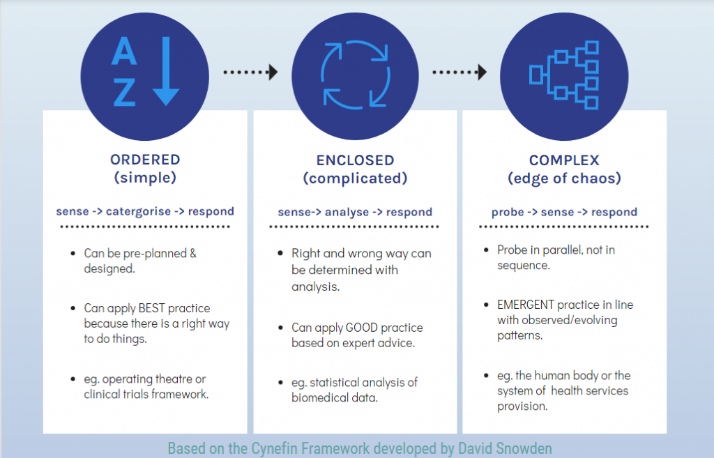
To further delineate the complex systems domain in practical terms we can use the Cynefin framework developed by David Snowden et al. to contrast the Simple, Complicated, Complex and Chaotic domains. For the purpose of this article the Chaotic domain will be ignored.

Enabling constraints of CAS models

In contrast to complex domain is the “known” or “simple” domain represented by ordered systems such as a surgical operating theatre or clinical trials framework. These ordered systems are rigidly constrained and can be planned and designed in advance based upon prior knowledge. In this context best practice can be applied because an optimal way of doing things is pre-determined.

The intermediary between the simple and complex domains is the “knowable” or ” complicated” domain. An example of such is the biostatistical analysis of basic clinical data. Within a complicated system there is a right answer that we can discover and design for. In this domain we can apply good practice based on expert advice (not best practice) as a right and wrong way of doing things can be determined with analysis.

Complex domain represents a system that is in flux and not predictable in the linear sense. A complex adaptive system can be operating in a state that is anywhere from equilibrium to the edge of chaos. In order to understand the system state one should perform experiments that probe relationships between entities. Due to the lack of linearity, multiple simultaneous experimental probes should occur in parallel, not in sequence, with the goal of better understanding processes. Emergent practice is determined in line with observed, evolving patterns. Ideally, decentralised Interpretation of data should be distributed to system users themselves rather than determined by a single expert in a centralised fashion.

As opposed to operating from a pre-supposed framework, the CAS structure should be allowed to emerge from the data under investigation. This avoids the confirmation bias that occurs when data are fitted to a predefined framework regardless of whether this framework best represents the data being modelled. Following on from this, model boundaries should also be allowed to emerge from the data itself.

Determining unarticulated needs from clusters of agent anecdotes or data points is a method of determining where improvement needs to occur in service provision systems. Yet this method forms an analogy that is mimicked in biological systems as well if an ABM was to be applied in a biomolecular context.

In understanding CAS, dispositionality of system states rather than linear causality should be the focus . Rather than presuming an inherent certainty as to “if I do A, B will result”, instead dispositional states arise as a result of A, which may result in B, but the evolution of which cannot be truly predicted.

“The longer you hold things in a state of transition the more options you’ve got” linear iterations based on a defined requirement with a degree of ambiguity which should be explored rather than eliminated. The opposite of standard statistical approach.

CAS modelling should include real-time feedback loops over multiple agents to avoid cognitive bias. In CAS modelling, every behaviour or interaction will produce unintended consequences, for this reason, David Snowden suggests, Small, fast experiments should be run in parallel, so that any bad, unintended consequences can be mitigated and the good ones amplified.

Modes of analysis and modelling:

System dynamics models (SDM)

  • A SDM simulates the movements of entities within the system and can be used to investigate macro behaviour of the system.
  • Changes to system state variables over time are modelled using differential equations.
  • SDMs are multi-dimentional, non-linear and include feedback mechanisms.

  • Visual representations of the model can be produced using stock and flow diagrams to summarise interdependencies between key system variables.
  • Dynamic hypotheses of the system model can be represented in a causal loop diagram
  • SDM is appropriate for modelling aggregate flows, trends, sub-system behaviour.

Agent based models (ABM)

  • ABMs can be used to investigate micro behaviour of the system from more of a bottom-up perspective through Intricate flows of individual based activity.
  • State changes of individual agents are simulated by ABMs rather than the broader entites captured by SDM
  • Multiple types of agent are operating within the same complex adaptive system modelled
  • Data within the ABM can be aggregated to infer more macro or top-down system behaviour.

Agents within the ABM can make decisions, engage in behaviour defined by simple rules and attributes, learn from experience and from feedback from interactions with other agents or the modelled environment. This is as true in models of human systems as it is with molecular scale systems. In both examples agents can par take in communication on a one to one, one to many and one to location basis. Previously popular models such as discrete event simulation (DES) was implemented to model passive agents at a finite time rather than active “decision makers” over dynamic periods that are a feature of ABMs.

Hybrid Models

  • Both ABM and SDM are complimentary techniques for simulating micro and macro level behaviour of complex adaptive systems and therefore engaging in exploratory style analysis of such systems.
  • Hybrid models emulate individual agent variability as well as variability in the the behaviour of aggregate entities they compose.
  • Simulate macro and micro level system behaviour in many areas of investigation such as health service provision, biomedical science.

Hybrid models have the ability to combine two or more types of simulation within the same model. These models can combine SDMs and ABMs, or other techniques, to address both top-down and bottom-up micro and macro dynamics in a single model that more closely captures whole system behaviour. This has the potential to elevate many of the necessary trade-offs of using one of the simulation types alone.

As software capability develops we are seeing an increased application of hybrid modelling techquiques. Previously wide-spread techniques such as DES and Markov models, which are one-dimentional, uni-directional, linear, are now proving inadequate in the task of modelling the complex adaptive and dynamic world we inhabit.

Model Validation Techniques

SDMs and ABMs are not fitted to observed data but instead use both qualitative and quantitative real world data to inform and develop the model and it’s parameters as a simulation of real world phenomena. For this reason model validation of SDMs and ABMs should be even more rigorous than for more traditional models such as maximum likelihood or least squares methods. Sensitivity analysis and validation tests such as behavioural validity tests can be used to compare model output against real-world data from organisations or experiments, relevant to the scale of the model being validated.

Structure of the model such as

  • Checking how the model behaves when subject to extreme parameter values.
  • Things like dimensional consistency, boundary adequacy, mass balance
  • Sensitivity analysis – how sensitive is the model to changes in key parameters.

Network Analysis

Data accrual from diverse data sources challenges and limitations

While complex systems theory has origins in the mathematics chaos theory, there are many examples contemporaneously where complex systems theory has been divorced form the mathematics and statistical modelling and applied in diverse fields such as business and healthcare or social services provision. Mathematical modelling adds validity to complex systems analysis. The problem with completing solely qualitative analysis without the empiricism of mathematical modelling, simulation and checking against a variety of real world data sets, the results

Complex Adaptive Systems (CAS) Approach to Biomedicine & Public Health

While a majority of biomedical and public health research still maintains a linear reductive approach to arrive at empiric insight, reality is in most cases neither of these things. A complex adaptive systems approach, like reality, is non-linear and high dimensional. There are many benefits from taking a linear cause-effect reductivist approach in that the complex problem and it’s solution becomes simplified into terms that can be understood and predicted.  Where this falls short is that predictions don’t often hold up in real world examples in which the outcomes tend to seem unpredictable.

Genomics, proteomics, transcriptomics and other “omics” techniques have generated an unprecedented amount of molecular genetics data. This data can be combined with larger scale data, from cell processes to environmental influences in disease states, to produce highly sophisticated multi-level models of contributing factors in human health and disease.

An area that is currently seeing an evolution into a more personalised nuanced approach, albeit still linear, is clinical trials. By introducing a biomarker component to clinical trials, for example to evaluate drug efficacy, the number of dimensions to the problem is slightly increased in order to arrive at more targeted and accurate solutions. More specifically, the number of patient sub-categories in the clinical trials increases to accommodate various biomarker groups which may respond more of less well to a different pharmacological approach to the same disease. Increasing the dimensions of the problem beyond this would, for now not be feasible or even helpful. On the other hand, understanding the interplay between biomolecular processes and environmental interactions in order to gain insight into disease processes themselves and thereby, which biochemical pathways for oncology drugs to target, is something that clearly benefits from a non-linear approach.

Another example of a system that benefits from a non-linear approach is public health service provision and the desire to garner insights into changes that increase prevention, early intervention and treatment effectiveness as well as reduce service cost for the government and patient. Both of the above examples require attention to both macro and micro processes.

Some components of complex adaptive systems: Connectivity, self organisation, emergent, fractal patterns, non-linear, governed by feedback loops, adaptive, nested systems, stochastic, simple rules, chaotic behaviour, iteration, sub optimal, requisite variety, may be considered optimised at the edge of chaos.

Whether modelling clinical health services networks or biological processes, complex adaptive systems consist of several common characteristics.

Components of complex adaptive systems

Massive interdependencies and elaborate connectivity

The complex adaptive systems approach shifts emphasis away from studying individual parts (such as seen in conventional medical science which produces notably fragmented results) to characterising the organisation of these parts in terms of their inherently dynamic interactions. CAS are open rather than closed systems because it is exogenous elements impacting on the system that cause the disruption required for growth.

Complex adaptive systems can be understood by relations and networks. System processes occur in networks that link component entities or agents. This approach emphasises that structures are dynamic and it is the process of becoming rather than the being itself that is of empirical interest.

Necessarily transdisciplinary or multi-disciplinary

A complex adaptive systems approach requires a transdisciplinary approach. The collaboration of numerous disparate experts is required in the combining of myriad biological, physical and societal based sciences into a holistic model. This model should aim to represent pertinent simultaneous top-down and bottom up processes that reveal contexts and relationships within the observed system dynamics.

Self-organising, emergent behaviour

Complex adaptive systems are selt-organising in the sense that observed patterns are open ended, potentially unfinished and cannot be predicted by the conventional definition. Rules of cause and effect are context dependent and can’t be applied in a rigid sense.

A self organising dynamic structure, which can be identified as a pattern, emerges as a result of individual spontaneous interactions between individual agents or elements. This pattern then impacts the interactions of individuals in a continual top down, bottom up symbiosis.

While linear models represent a reductionist, closed conceptualisation of the phenomena under analysis, a complex systems approach embraces high dimensionality true to the myriad real world phenomena composing a system. This requires that the system be treated as open and of uncertain ontology and thus lacking predictive capacity with regards to the outcomes of system dynamics.

As an emergent phenomena, the complex adaptive system can be understood by interacting with it rather than through analysis or static modelling. This approach is concerned with “state change” or to evaluate “how things are becoming”, rather than “how thing are”. How did today’s state emerge from yesterday’s trajectories and process dynamics?

Fractal engagement. Fractal engagement entails that the system as a whole orientates through multiple actions. The same data can produce frameworks at the level of responsibility of every individual agent. Using public health intervention as an example, Individual agents make decisions, based on the data, as to what changes they can make tomorrow within their own sphere of competence, rather than overarching changes being dictated and determined in a top down way, or by others.

Feedback loops

Feedback loops link individual parts into an overaching dynamic structure. Feedback loops are self-reinforcing and can be positive or negative.

Negative feedback loops are stabalising in that they have a dampening effect on oscillations that causes the system or component to move closer to equilibrium. Positive feedback loops are morphogenic and increase the frequency and amplitude of oscillations driving the system away from homeostasis and leading to changes in the underlying structure or the system.

Positive feedback loops, while facilitating growth and adaptation, tend towards chaos and decay and are thus crucially counterbalanced by simultaneously operating negative feedback loops. Evolution is supposed to occur as a series of phase transitions, back and forth, from ordered to disordered states.

Both top-down and bottom-up “causality”

While CAS models describe elements in terms of possibilities and probabilities, rather than cause and effect in the linear sense, there is a clear interplay between top down and bottom up causality and influence on the dynamic flows and trajectories of any system. This is very much a mirror of real world systems. One example of this is the human body where both conscious thought (top down) and biomolecular processes such as hormonal and neurochemical fluctuations (bottom up) effect mood, which in turn has a lot of flow on effects down stream that cause changes that shirt the system back and forth from health to disease. One such manifestation of this is stress induced illness of various kinds. As a social example, we can of course find many examples of top down and bottom up causation in a public heath or epidemiological setting.

This has been a non-exhaustive description of just some key components of complex adaptive systems. The main purpose is to differentiate the CAS paradigm from the more mainstream biomedical research paradigm and approach. For a deeper dive into the concepts mentioned see the references below.

References:

https://core-cms.prod.aop.cambridge.org/core/services/aop-cambridge core/content/view/F6F59CA8879515E3178770111717455A/9781108498692c7_100-118.pdf/role_of_the_complex_adaptive_systems_approach.pdf

Carmichael T., Hadžikadić M. (2019) The Fundamentals of Complex Adaptive Systems. In: Carmichael T., Collins A., Hadžikadić M. (eds) Complex Adaptive Systems. Understanding Complex Systems. Springer, Cham. https://doi.org/10.1007/978-3-030-20309-2_1

https://www.health.org.uk/sites/default/files/ComplexAdaptiveSystems.pdf

Milanesi, L., Romano, P., Castellani, G., Remondini, D., & Liò, P. (2009). Trends in modeling Biomedical Complex Systems. BMC bioinformatics10 Suppl 12(Suppl 12), I1. https://doi.org/10.1186/1471-2105-10-S12-I1

Sturmberg J. P. (2021). Health and Disease Are Dynamic Complex-Adaptive States Implications for Practice and Research. Frontiers in psychiatry12, 595124. https://doi.org/10.3389/fpsyt.2021.595124

Master Protocols for Clinical Trials

Part 1: Basket & Umbrella Trial Designs

Introduction

As the clinical research landscape becomes ever more complex and interdisciplinary alongside an evolving genomic and biomolecular understanding of disease, the statistical design component that underpins this research must adapt to accommodate this. Accuracy of evidence and speed with which novel therapeutics are brought to market remain hurdles to be surmounted.

While efficacy studies or non-inferiority clinical trials in the drug development space traditionally only included broad disease states usually with patients randomised to a dual arm of new treatment compared to an existing standard treatment. Due to patient biomarker heterogeneity, effective treatments could be left unsupported by evidence. Similarly treatments found effective in a clinical trial don’t always translate to show real world effectiveness in a broader range of patients.

Our current ability to assess individual genomic, proteomic and transcriptomic data and other patient bio-markers for disease, as well as immunologic and receptor site activity, has shown that different patients respond differently to the same treatment and, the same disease may benefit from different treatments in different patients – thus the beginnings of precision medicine.  In addition to this is the scenario where a single therapeutic may be effective against a number of different diseases or subclasses of a disease based on the agent’s mechanism of action on molecular processes common to the disease states under evaluation.

Master protocols, or complex innovative designs, are designed to pool resources to avoid redundancy and test multiple hypotheses under one clinical trial, rather than multiple clinical trials being carried out separately over a longer period of time.

Due to this fairly novel evolution in the clinical research paradigm and also due to inherent flexibility within each study design, conflicting information related to the definition and characterisation of master protocols such as basket and umbrella clinical trials as well as cases in the published literature where the terms “basket” and “umbrella” trials have been used interchangeably or are ill-defined exists. For this reason a brief definition and overview of basket and umbrella clinical trials is included in the paragraphs that follow. Based on systematic reviews of existing research it seeks the clarity of consensus, before detailing some key statistical and operational elements of each design.

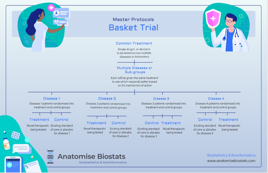
Master protocols for bio-marker based clinical trials.
Diagram of a basket trial design.

Basket trial:

A basket clinical trial design consists of a targeted therapy, such as a drug or treatment device, that is being tested on multiple disease states characterised by a common molecular process that is impacted by the treatment’s mechanism of action. These disease states could also share a common genetic or proteomic alteration that researchers are looking to target.

Basket trials can be either exploratory or confirmatory and range from full randomised, controlled double-blinded designs to single arm designs, or anything in between. Single arm designs are an option when feasibility is limited and are more focused on the pre-clinical stage of determining efficacy or whether a particular treatment has clear-cut commercial potential evidenced by a sizable enough retreat in disease symptomology. Depending on the nuances of the patient populations being evaluated final study data may be analyses by pooling disease states or by each disease state separately. Basket trials allow drug development companies to target the lowest hanging fruit in terms of treatment efficacy, focusing resources on therapeutics with the highest potential of success in terms of real patient outcomes.

Master protocol umbrella trial
Diagram of an umbrella trial design.

Umbrella trial:

An umbrella clinical trial design consists of multiple targeted treatments of a single disease where patients can be sub-categorised into biomarker subgroups defined by molecular characteristics that may lend themselves to one treatment over another.

Umbrella trials can be randomised, controlled double-blind studies that in which each intervention and control pair is analysed independently of other treatments in the trial, or where feasibility issues dictate, they can be conducted without a control group with results analysed together in-order to compare the different treatments directly.

Umbrella trials may be useful when a treatment has shown efficacy in some patients and not others, they increase the potential for confirmatory trial success by honing in on patient sub-populations that are most likely to benefit due to biomarker characteristics, rather than grouping all patients together as a whole.

Basket & Umbrella trials compared:

Both basket and umbrella trials are typically biomarker guided. The difference being that basket trials aim to evaluate tissue-agnostic treatments to multiple diseases based on common molecular characteristics, whereas umbrella trials aim to evaluate nuanced treatment approaches to the same disease based on differing molecular characteristics between patients.

Biomarker guided trials have an additional feasibility constraint to non-biomarker guided trials in that the size of the eligible patient pool is reduced in proportion to the prevalence of the biomarker/s of interest within that patient pool. This is why master protocol methodology becomes instrumental in enabling these appropriately complex research questions to be pursued.

Statistical Concepts and considerations of basket and umbrella Trials

Effect size

Basket and umbrella trials generally require a larger effect size than traditional clinical trials, in order to achieve statistical significance. This is in a large part due to the smaller sample sizes and higher variance that comes with that. While patient heterogeneity in terms of genomic or molecular diversity, and thus expected treatment outcome, has been reduced by the precision targeting of the trial design, there is a certain degree of between-patient heterogeneity that can only be expected when relying on treatment arms of very small sample sizes.

If resources, including time, are tight then basket trials enable drug developers to focus on less risky treatments that are more likely to end in profitability. It should be noted that this does not always mean that the treatments that are rejected by basket trials are truly clinically ineffective. A single arm exploratory basket trial could end up rejecting a potential new treatment that, if subject to a standard trial with more drawn out patient acquisition and a larger sample size, would have been deemed effective at a narrower effect size.

Screening efficiency

If researchers carry out separate clinical studies for each biomarker of interest, then a separate screening sample needs to be recruited for each study. The rarer the biomarker, the larger the recruited screening sample would need to find enough people with the biomarker to participate in the study. This number needs to be multiplied by the number of biomarkers. A benefit of master protocols is that a single sample of people can be screened for multiple biomarkers at once, greatly reducing the required screening sample size.

 For example, researchers interested in 4 different biomarkers could collectively reduce the required screening sample by three quarters compared to conducting separate clinical studies for each biomarker. This maximisation of resources can be particularly helpful when dealing with rare biomarkers or diseases.

Patient allocation considerations

If relevant biomarkers are not mutually exclusive a patient could fit into multiple biomarker groups for which treatment is being assessed in the study. In this scenario a decision has to be made as to which category the patient will be assigned and the decision process may occur at random where appropriate. If belonging to two overlapping biomarker groups is problematic in terms of introducing bias in small sample sizes, or if several patients have the same overlap, then a decision may be made to collapse the two biomarkers into a single group or eliminate one of the groups. If a rare genetic mutation is a priority focus in the study then feasibility would dictate that the patient be assigned to this biomarker group.

Sample Size calculations

Generally speaking, sample size calculation for basket trials should be based on the overall cohort, whereas sample size calculations for umbrella trials are typically undertaken individually for each treatment.

Basket and umbrella trials can be useful in situations where a smaller sample size is more feasible due to specifics of the patient population under investigation. Statistically designing for this smaller sample size typically comes at the cost of necessitating a greater effect size (difference between treatment and control) and this translates to lower overall study power and greater chance of type 1 error (false negative result) when compared to a standard clinical trial design. Despite these limitations master protocols such as basket or umbrella trials allow to evaluation of certain treatments to the highest possible level of evidence that otherwise might be too heterogeneous or rare to evaluate using a traditional phase II or III trial.

Randomisation and control

Randomised controlled designs are recommended for confirmatory analysis of an established treatment or target of interest. The control group typically treats patients with the established standard of care for their particular disease or, in the absence of one, placebo.

In master basket trials the established standard of care is likely to differ by disease or disease sub-type. For this reason it may be necessary for randomised controlled basket trials pair a control group with each disease sub-group rather than just incorporating a single overall control group and potentially pooling results from all diseases under one statistical analysis of treatment success. Instead it is worth considering if each disease type and corresponding control pair could be analysed separately to enhance statistical robustness in a truly randomised controlled methodology.

Single arm (non-randomised designs) are sometimes necessary for exploratory analysis of potential treatments or targets. These designs often require a greater margin of success (treatment efficacy) to be statistically significant as a trade-off for a smaller sample size required.

Blinding

To increase the quality of evidence, all clinical studies should be double blinded where possible.

To truly evaluate the effectiveness of a treatment without undue bias from a statistical perspective double-blinding is recommended.

Aside from increased risk of type 2 error that may be inherent in master protocol designs, there is a greater potential for statistical bias to be introduced. Bias can introduce itself in a myriad of ways and results in a reduction in the quality of evidence that a study can produce. Two key sources of bias are lack of randomisation (mentioned above) and lack of blinding.

Single armed trials do not include a control arm and therefore patients cannot be randomised to a treatment arm where double-blinding of patients, practitioners, researchers and data managers etc will prevent various types of bias creeping in to influence the study outcomes. With so many factors at play it is important not to overlook the importance of study blinding and implement it whenever feasible to do so.

If the priority is getting a new treatment or product to market fast to benefit patients and potentially save lives, accommodating this bias can be a necessary trade-off. It is after-all typically quite a challenge to have clinical data and patient populations that are at homogeneous and matched to any great degree, and this reality is especially noticeable with rare diseases or rare biomarkers.

Biomarker Assay methodology

The reliability of biologic variables included in a clinical trial should be assessed, for example the established sensitivity and specificity of particular assays needs to be taken into account. When considering patient allocation by biomarker group, the degree of potential inaccuracy of this allocation can have a significant impact on trial results, particularly when there is a small sample size. If the false positive rate of a biomarker assay is too high this will result in the wrong patients qualifying for treatment arms, in some cases this may reduce the statistical power of the study.

A further consideration of assay methodology pertains to the potential for non-uniform bio-specimen quality at different collection sites which may bias study results. A monitoring framework should be considered in order to mitigate this.

Patient tissue samples required for assays, can inhibit feasibility and increase time and cost in the short term and make study reproducibility more complicated. While this is important to note these techniques are in many cases necessary in effectively assessing treatments based on our contemporary understanding a many disease states such as cancer within the modern oncology paradigm. Without incorporating this level of complexity and personalisation into clinical research it will not be possible to develop evidence based treatments that translate into real-world effectiveness and thus widespread positive outcomes for patients.

Data management and statistical analysis

The ability to statistically analyse multiple research hypotheses at once within a single dataset increases efficiency at the biostatisticians end and allows frameworks for greater reproducibility of the methodology and final results, compared to the execution and analysis of multiple separate clinical trials testing the same hypotheses. Master protocols also enable increased data sharing and collaboration between sites and stakeholders.

Deloitte research estimated that master protocols can save clinical trials 12-15% in cost and 13-18% in study duration. These savings of course apply to situations where master protocols were a good fit for the clinical research context, rather than to the blanket application of these study designs across any or all clinical studies. Applying a master protocol study design to the wrong clinical study could actually end up increasing required resources and costs without benefit, therefore it is important to assess whether a master protocol study design is indeed the optimal approach for the goals of a particular clinical study or studies.

umbrella trials for precision medicine
Master protocols for precision medicine.

References:

Bitterman DS, Cagney DN, Singer LL, Nguyen PL, Catalano PJ, Mak RH. Master Protocol Trial Design for Efficient and Rational Evaluation of Novel Therapeutic Oncology Devices. J Natl Cancer Inst. 2020 Mar 1;112(3):229-237. doi: 10.1093/jnci/djz167. PMID: 31504680; PMCID: PMC7073911.

Lesser N, Na B, Master protocols: Shifting the drug development paradigm, Deloitte Center for Health solutions

Lai TL, Sklar M, Thomas, N, Novel clinical trial solutions and statistical methods in the era of precision medicine, Technical Report No. 2020-06, June 2020

Renfro LA, Sargent DJ. Statistical controversies in clinical research: basket trials, umbrella trials, and other master protocols: a review and examples. Ann Oncol. 2017 Jan 1;28(1):34-43. doi: 10.1093/annonc/mdw413. PMID: 28177494; PMCID: PMC5834138.

Park, J.J.H., Siden, E., Zoratti, M.J. et al. Systematic review of basket trials, umbrella trials, and platform trials: a landscape analysis of master protocols. Trials 20, 572 (2019). https://doi.org/10.1186/s13063-019-3664-1

Distributed Ledger Technology for Clinical & Life Sciences Research: some Use-Cases for Blockchain & Directed Acyclic Graphs

Applications of blockchain and other distributed ledger technology (DLT) such as directed acyclic graphs (DAG) to clinical trials and life sciences research are rapidly emerging.

Distributed ledger technology (DLT) such as blockchain has a myriad of use-cases in life sciences and clinical research.
Distributed ledger technology (DLT) has the potential to solve a myriad of problems that currently plague data collection, management and access processes in clinical and life sciences research, including clinical trials. DLT is an innovative approach to operating in environments where trust and integrity is paramount by paradoxically removing the need for trust in any individual component and providing full transparency as to the micro-environment of the platform operations as a whole.Currently the two forms of DLT predominating are blockchain and directed acyclic graphs (DAGs). While quite distinct from one another, in theory the two technologies are intended to serve similar purposes, or were developed to address the same goals. In practice, blockchain and DAGs may have optimal use-cases that differ in nature from one another, or be better equipped to serve different goals – the nuance of which to be determined on a case by case basis.

Bitcoin is the first known example of blockchain, however blockchain goes well beyond the realms of bitcoin and cryptocurrency use cases. One of the earliest and currently predominating DAG DLT platforms is IOTA which has proved itself in a plethora of use cases that go well beyond what blockchain could currently achieve, particularly within the realm of the internet of things (IOT). In fact Iota has been developing an industry data marketplace active since 2017 which makes it possible to store, sell via micro-transactions and access data streams via web browser. For the purposes of this article we will focus on DLT applications in general and include use-cases in which blockchain or DAGs can be employed interchangeably. Before we begin, what is Distributed Ledger  technology?

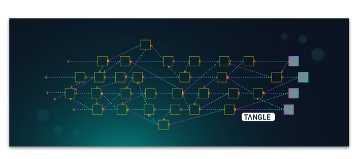
The Iota Tangle has already been implemented in a plethora of use cases that may be beneficially translated to clinical and life sciences research.

Source: iota.org Iota’s Tangle is an example of directed acyclic graph (DAG) digital ledger technology. Iota has been operating an industry data marketplace since 2017.
​DLT is a decentralised digital system which can be used to store data and record transactions in the form of a ledger or smart contract. Smart contracts can be set up to form a pipeline of conditioned (if-then) events, or transactions, much like an escrow in finance, which are shared across nodes on the network. Nodes are used to both store data and process transactions, with multiple (if not all) nodes accommodating each transaction – hence the decentralisation. Transactions themselves are a form of dynamic data, while a data set is an example of static data. Both blockchain and DAGs employ advanced cryptography algorithms which as of today render them un-hackable. This is a huge benefit in the context of sensitive data collection such as patient medical records or confidential study data. It means that data can be kept secure, private, untampered with, and shared efficiently with whomever requires access. Because each interaction or transaction is recorded this enables the integrity of the data to be upheld in what is considered a “trustless” exchange. Because data is shared on multiple nodes for all involved to witness across the network, records become harder to manipulate of change in an underhanded way. This is important in the collection of patient records or experimental data that is destined for statistical analysis. Any alterations to data that are made are recorded across the network for all participants to see, enabling true transparency. All transactions can come in the form of smart contracts which are time stamped and tied to a participant’s identity via the use of digital signatures.

In this sense DLT is able to speed up transactions and processes, while reducing cost, due to the removal of a middle-man or central authority overseeing each transaction, or transfer of information. DLT can be public or private in nature. A private blockchain, for example, does have trusted intermediary who decides who is to have access to the blockchain, who can participate on the network, which data can be viewed by which participants. In the context of clinical and life sciences research this could be a consortium of interested parties, ie the research team, or an industry regulator or governing body. In a private blockchain, the transactions themselves remain decentralised, while the blockchain itself has built in permission layers that allow full or partial visibility of data depending upon the stakeholder. This is necessary in the context of sharing anonymised patient data and blinding in randomised controlled trials.
Blockchain and Hashgraph are two examples of distributed ledger technology (DLT) with applications which could achieve interoperability across healthcare,  medicine, insurance, clinical trials and life sciences research.

Source: Hedera Hashgraph whitepaper. Blockchain and Hashgraph are two examples of distributed ledger technology (DLT).
Due to the immutable nature of each ledger transaction, or smart contract, stakeholders are unable to alter or delete study data without a consensus over the whole network. In this situation, an additional transaction recorded and time-stamped on the blockchain while the original transaction, that recorded the data to be altered in its original form, remains intact. This property helps to reduce the incidence of human error, such as data entry error, as well as any underhanded alterations with the potential to sway study outcomes.

In a clinical trials context the job of the data monitoring committee, and any other form of auditing  becomes much more straight forward. DLT also allow for complete transparency in all financial transactions associated with the research. Funding bodies can see exactly where all funds are being allocated and at what time points. In-fact every aspect of the research supply-chain, from inventory to event tracking, can be made transparent to the desired entities. Smart contracts operate among participants in the blockchain and also between the trusted intermediary and the DLT developer whose services have been contracted for building the platform framework, such as the private blockchain. The services contracts will need to be negotiated in advance so that the platform is tailored to adequately conform to individualised study needs. Once processes are in place and streamlines the platform can be replicated in comparable future studies.

DLT can address the problem of duplicate records in study data or patient records, make longitudinal data collection more consistent and reliable across multiple life cycles. Many disparate stakeholders, from doctor to insurer or researcher, can share in the same patient data source while maintaining patient privacy and improving data security. Patients can retain access to the data and decide with whom to share it with, which clinical studies to participate in and when to give or withdraw consent.

DLT, such as blockchain or DAGs, can improve collaboration by making the sharing of technical knowledge easier and centralising data or medical records, in the sense that they are located on the same platform as every other transaction taking place. This results in easier shared access by key stakeholders, shortening of negotiation cycles due to improved coordination and making established clinical research processes more consistent and replicable.

From a statisticians perspective, DLT should result in data of higher integrity which yields statistical analysis of greater accuracy and produces research with more reliable results that can be better replicated and validated in future research. Clinical studies will be streamlined due to the removal of much bureaucracy and therefore more time and cost effective to implement as a whole. This is particularly important in a micro-environment with many moving parts and disparate stakeholders such as the clinical trials landscape.


References and further reading:

From Clinical Trials to Highly Trustable Clinical Trials: Blockchain in Clinical Trials, a Game Changer for Improving Transparency?
https://www.frontiersin.org/articles/10.3389/fbloc.2019.00023/full#h4

Clinical Trials of Blockchain

Blockchain technology for improving clinical research quality
https://trialsjournal.biomedcentral.com/articles/10.1186/s13063-017-2035-z

Blockchain to Blockchains in Life Sciences and Health Care
https://www2.deloitte.com/content/dam/Deloitte/us/Documents/life-sciences-health-care/us-lshc-tech-trends2-blockchain.pdf

Simpson’s Paradox: the perils of hidden bias.

How Simpson’s Paradox Confounds Research Findings And Why Knowing Which Groups To Segment By Can Reverse Study Findings By Eliminating Bias.

Introduction
 
The misinterpretation of statistics or even the “mis”-analysis of data can occur for a variety of reasons and to a variety of ends. This article will focus on one such phenomenon
contributing to the drawing of faulty conclusion from data – Simpson’s Paradox.


At times a situation arises where the outcomes of a clinical research study depict the inverse of expected (or essentially correct) outcomes. Depending upon the statistical approach, this could affect means, proportions or relational trends among other statistics.
Some examples of this occurrence are a negative difference when a positive difference was anticipated, a positive trend when a negative one would have been more intuitive – or vice versa. Another example commonly pertains to the cross tabulation of proportions, where condition A is proportionally greater over all, yet when stratified by a third variable, condition B is greater in all cases . All of these examples can be said to be instances of Simpson’s paradox. Essentially Simpson’s paradox represents the possibility of supporting opposing hypotheses – with the same data.
Simpson’s paradox can be said to occur due to the effects of confounding, where a confounding variable is characterised by being related to both the independent variable and the outcome variable, and unevenly distributed across levels of the independent variable. Simpson’s paradox can also occur without confounding in the context of non-collapsability. 
For more information on the nuances of confounding versus non-collapsability in the context of Simpson’s paradox, see here.

 In a sense, Simpson’s paradox is merely an apparent paradox, and can be more accurately described as a form of bias. This bias most often results from a lack of insight into how an unknown lurking variable, so to speak, is impacting upon the relationship between two variables of interest. Simpson’s paradox highlights the fact that taking data at face value and utilising it to inform clinical decision making can often be highly misleading. The chances of Simpson’s paradox (or bias) impacting the statistical analysis can be greatly reduced in many cases by a careful approach that has been informed by proper knowledge of the subject matter. This highlights the benefit of close collaboration between researcher and statistician in informing an optimal statistical methodology that can be adapted on a per case basis.

The following three part series explores hypothetical clinical research scenarios in which Simpson’s paradox can manifest.

Part 1

Simpson’s Paradox in correlation and linear regression

​​

​Scenario and Example

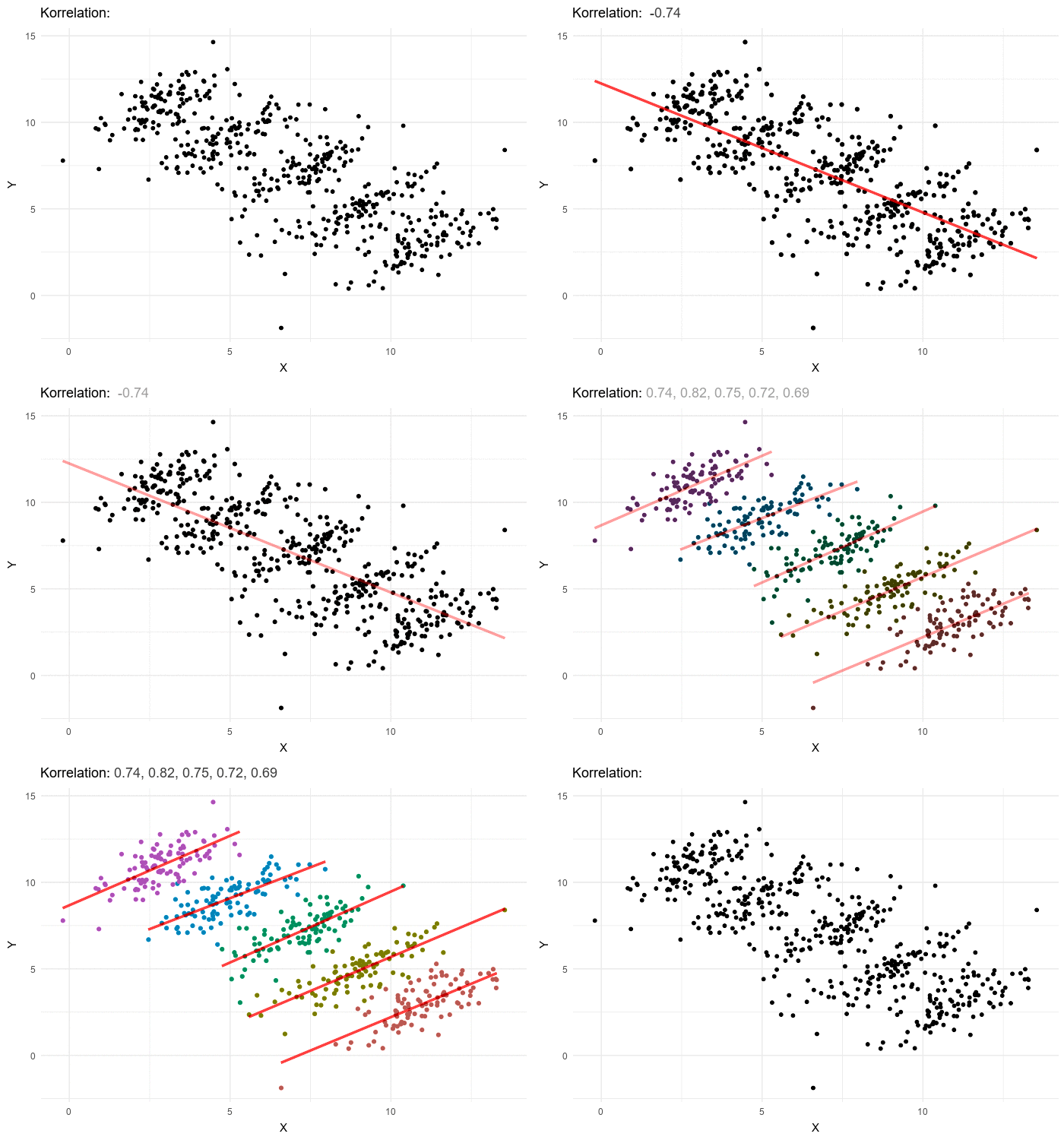
A nutritionist would like to investigate the relationships between diet and negative health outcomes. As higher weight has been previously associated with negative health outcomes, the research sets out to investigate the extent to which increased caloric intake contributes to weight gain. In researching the relationship between calorie intake and weight gain for a particular dietary regime, the nutritionist uncovers a rather unanticipated negative trend. As caloric intake increases the weight of participants appears to go down. The nutritionist therefore starts recommending higher calorie intake as a way to dramatically lose weight. Weight does appear to go down with calorie intake, however if we stratify the data by different age groupings, a positive trend between weight and calorie intake emerges for each age group. While overall elderly have the lowest calorie intake, they also have the highest weight, and teens have the highest calorie intake but the lowest weight, this accounts for the negative trend but does not give an honest picture of the impact of calories on weight. In order to gain an accurate picture of the relationship between weight and calorie intake we have to know which variable to group or stratify the data by, and in this case it’s age. Once the data is stratified by five separate age categories a positive trend between calories and weight emerges in each of the 5 categories. In general, the answer to which variable to stratify by or control for isn’t typically this obvious and in most cases and requires some theoretical background and a thorough examination of the available data including associated variables for which the information is at hand.


Remedy

In the above example, age shows a negative relationship to the independent variable, calories, but a positive relationship to the dependent variable, weight. It is for this reason that a bit of data exploration and assumption checking before any hypothesis testing is so essential. Even with these practices in place it is possible to overlook the source of confounding and caution is always encouraged.
 
Randomisation and Stratification:
In the context of a randomised controlled trial (RTC), the data should be randomly assigned to treatment groups as well as stratified by any pertinent demographic and other factors so that these are evenly distributed across treatment arms (levels of the independent variable). This approach can help to minimise, although not eliminate the chances of bias occurring in any such statistical context, predictive modelling or otherwise.

Linear Structural Equation Modelling:
 If the data at hand is not randomised but observational, a different approach should be taken to detect causal effects in light of potential confounding or non-collapsability. One such approach is linear structural equation modelling where each variable is generated as a linear function of it’s parents, using a directed acyclic graph (DAG) with weighted edges. This is a more sophisticated and ideal approach to simply adjusting for x number of variables, which is needed in the absence of a randomisation protocol.

Heirachical regression:
This example illustrated an apparent negative trend of the overall data masking a positive trend In each individual subgroup, in practice, the reverse can also occur.
In order to avoid drawing misguided conclusion from the data the correct statistical approach must be entertained, a hierarchical regression controlling for a number of potential confounding factors could avoid drawing wrong conclusion due to Simpson’s paradox.


Article: Sarah Seppelt Baker


Reference:
The Simpson’s paradox unraveled, Hernan, M, Clayton, D, Keiding, N., International Journal of Epidemiology, 2011.

Part 2

Simpson’s Paradox in 2 x 2 tables and proportions


​Scenario and Example

Simpson’s paradox can manifest itself in the analysis of proportional data and two by two tables. In the following example two pharmaceutical cancer treatments are compared by a drug company utilising a randomised controlled clinical trial design. The company wants to test how the new drug (A) compares to the standard drug (B) already widely in clinical use.  1000 patients were randomly allocated to each group. A chi squared test of remission rates between the two drug treatments is highly statistically significant, indicating that the new drug A is the more effective choice. At first glance this seems reasonable, the sample size is fairly large and equal number of patients have been allocated to each groups.
Drug  Treatment
A
B
Remisson Yes
798 (79.8%)
705 (70.5%)
Remission No
202
295
Total sample size
1000
1000
The chi-square statistic for the difference in remission rates between treatment groups is 23.1569. The p-value is < .00001. The result is significant at p < .05.


When we take a closer look, the picture changes. It turns out the clinical trial team forgot to take into account the patients stage of disease progression at the commencement of treatment. The table below shown that drug A was allocated to far more patients with stage II cancer (79.2%) and drug B was allocated to far more patients with stage IV cancer (79.8%). 

Stage II
Stage IV
Drug Treatment
A
B
A
B
Remission Yes
697 (87.1%)
195 (92.9%)
101 (50.5%)
510 (64.6%)
Remission No
103
15
99
280
Total sample size
800
210
200
790
The chi-square statistic for the difference in remission rates between treatment groups for patients with stage II disease progression at treatment outset is 5.2969. The p-value is .021364. The result is significant at p < .05.


The chi-square statistic for the difference in remission rates between treatment groups for patients with stage IV disease progression at treatment outset is 13.3473. The p-value is .000259. The result is significant at p < .05.

Unfortunately the analysis of tabulated data is no less prone to bias in results akin to Simpson’s Paradox than continuous data. Given that stage II cancer is easier to treat than stage IV, this has given drug A an unfair advantage and has naturally lead to a higher remission rate overall for drug A. When the treatment groups are divided by disease progression categories and reanalysed, we can see that remission rates are higher for drug B in both stage II and stage IV baseline disease progression. The resulting chi squared statistics are wildly different to the first and statistically significant in the opposite direction to the first analysis.  In causal terms, stage of disease progression affects difficulty of treatment and likelihood of remission. Patients at a more advanced stage of disease, ie stage IV, will be harder to treat than patients at stage II. In order for a fair comparison between two treatments, patients stage of disease progression needs to be taken into account. In addition to this some drugs may be more efficacious at one stage or the other, independent of the overall probabilities of achieving remission at either stage. 

Remedy

Randomisation and Stratification:
Of course in this scenario, stage of disease progression is not the only variable that needs to be accounted for in order to insure against biased results. Demographic variables such as age, sex socio-economic status and geographic location are some examples of variables that should be controlled for in any similar analysis. As with the scenario in part 1, this can be achieved is through stratified random allocation of patients to treatment groups at the outset of the study. Using a randomised controlled trial design where subjects are randomly allocated to each treatment group as well as stratified by pertinent demographic and diagnostic variables will reduce the chances of inaccurate study results occurring due to bias.

Further examples of Simpson’s Paradox in 2 x 2 tables

Simpson’s paradox in case control and cohort studies

Case control and cohort studies also involve analyses which rely on the 2×2 table. The calculation of their corresponding measures of association the odds ratio and relative risk, respectively, is unsurprisingly not immune to the effect of bias and in much the same way as the chi square example above. This time, a reversed odds ratio or relative risk in the opposite direction can occur if the pertinent bias has not been accounted and controlled for.

Simpson’s paradox in meta-analysis of case control studies

Following on from the example above, this form of bias can pose further problems in the context of meta-analysis. When combining results from numerous case control studies the confounders in question may or may not have been identified or controlled for consistently across all studies and some studies will likely have identified different confounders to the same variable of interest. The odds ratios produced by the different studies can therefore be incompatible and lead to erroneous conclusions. Meta-analysis can therefore fall prey to ecological fallacy as a result of systematic bias, where the odds ratio for the combined studies is in the opposite direction to the odds ratios of the separate studies. Imbalance in treatment arm size has also been found to act as a confounder in the context of meta-analysis of randomised controlled trials. Other methodological differences between studies may also be at play, such as differences in follow-up times between studies or a very low proportion of observed events occurring in some studies, potentially due to a shorted follow-up time.

That’s not to say that meta-analysis cannot be performed on these studies, inter-study variation is of-course more common than not, as with all other analytical contexts it is necessary to proceed with a high level of caution and attention to detail. On the whole an approach of simply pooling study results is not reliable, the use of more sophisticated meta-analytic techniques, such as random effects models or Bayesian random effects models that use a Markov chain algorithm for estimating the posterior distributions, are required to mitigate inherent limitations of the meta-analytic approach. Random-effects models assume the presence of study-specific variance which is a latent variable to be partitioned. Bayesian random-effects models can come in parametric, non-parametric or semi-parametric varieties, referring to the shape of the distributions of study-specific effects.
​​
For more information on Simpson’s paradox in meta-analysis, see here.

https://bmcmedresmethodol.biomedcentral.com/articles/10.1186/1471-2288-8-34

For more information on how to minimise bias in meta-analysis, see here.

https://www.ncbi.nlm.nih.gov/pmc/articles/PMC3868184/

https://onlinelibrary.wiley.com/doi/abs/10.1002/sim.4780110202

Part 3

Simpson’s Paradox & Cox Proportional Hazard Models

Time to event data is common in clinical science and epidemiology, particularly in the context of survival analysis. Unfortunately the calculation of hazard rate in survival analysis is not immune to Simpson’s Paradox as the mathematics behind Simpson’s paradox is essentially the mathematics of conditional probability. In-fact Simpson’s paradox in this context has the interesting characteristic  of holding for some intervals of the time variable (failure time T) but not others. In this case Simpson’s paradox would be observed across the effect of variable Y on the relationship between variable X and time interval T. The proportional hazards model can be seen as an extension of 2 by 2 tables, given that the type of data is similar is used, the difference being that time is typically is as much an outcome of interest in relation to some factor Y. In this context Y could be said to be a covariate to X.

Scenario and example
 
A 2017 paper describes a scenario whereby the death rate due to tuberculosis was lower in Richmond than New York for both African-Americans and for Caucasian-Americans, yet lower in New York than Richmond when the two ethnic groups were combined.
For more details on this example as well as the mathematics behind it see here.
For more examples of Simpson’s paradox in Cox regression see here.


Site specific bias

Factors contributing to bias in survival models can be different to those in more straightforward contexts. Many clinical and epidemiological studies include data from multiple sites. More often than not there is heterogeneity across sites. This heterogeneity can come is various forms and can result in within and between–site clustering, or correlation, of observations on site specific variables. This clustering, if not controlled for, can lead to Simpson’s paradox in the form of hazard rate reversal, across some or all of time T, and has been found to be a common explanation of the phenomenon in this context. Site clustering can occur on the patient level, for example, due to site specific selection procedures for the recruitment of patients (lead by the principal investigators individual to each site), or differences in site specific treatment protocols. Site specific differences can occur intra or internationally and in the international case can be due, for example, to differences in national treatment guidelines or differences in drug availability between countries. Resource availability can also differ between sites whether intra or internationally. In any time to event analysis involving multiple sites (such as the Cox regression model) a site-level effect should be taken into account and controlled for in order to avoid bias-related inferential errors.


Remedy
 

Cox regression Model including site as a fixed covariate:
Site should be included as a covariate in order to account for site specific dependence of observations.

Cox regression Model treating site as a stratification variable:
In cases where one or more covariates violate the Proportional Hazards (PH) assumption as indicated by a lack of independence of scaled Schonefeld residuals to time, stratification may be more appropriate. Another option in this case is to add a time-varying covariate to the model. The choice made in this regard will depend on the sampling nuances of each particular study.

Cox shared frailty model:
In specific conditions the Cox shared frailty model may be more appropriate. This approach involves treating subjects from the same site as having the same frailty and requires that each subjects is not clustered across more than one level two unit. While it is not appropriate for multi-membership multi-level data, it can be useful for more straight forward scenarios.

In tailoring the approach to the specifics of the data, appropriate model adjustments should produce hazard ratios that more accurately estimate the true risk.

Latent Variable Modelling And The Chi Squared Exact Fit Statistic

Latent variable modelling and the chi squared exact fit statistic

Latent variable models are exploratory statistical models used extensively throughout clinical and experimental research in medicine and the life sciences in general. Psychology and neuroscience are two key sub-disciplines where latent variable models are routinely employed to answer a myriad of research questions from the impact of personality traits on success metrics in the workplace (1) to measuring inter-correlated activity of neural populations in the human brain based on neuro-imaging data (2). Through latent variable modelling, dispositions, states or process which must be inferred rather than directly measured can be linked causally to more concrete measurements.
Latent variable models are exploratory or confirmatory in nature in the sense that they are designed to uncover causal relationships between observable or manifest variables and corresponding latent variables in an inter-correlated data set. They use structural equation modelling (SEM) and more specifically factor analysis techniques to determine these causal relationships which and allow the testing of numerous multivariate hypotheses simultaneously. A key assumption of SEM is that the model is fully correctly specified. The reason for this is this is that one small misspecification can affect all parameter estimations in the model, rendering inaccurate approximations which can combine in unpredictable ways (3).

With any postulated statistical model it is imperative to assess and validate the model fit before concluding in favour of the integrity of the model and interpreting results. The acceptable way to do this across all structural equation models is the chi squared (χ²) statistic.

A statistically significant χ² statistic is indicative of the following:

  • A systematically miss-specified model with the degree of misspecification a function of the χ² value.
  • The set of parameters specified in the model do not adequately fit the data and thus that the parameter estimates of the model are inaccurate. As χ² operates on the same statistical principles as the parameter estimation, it follows that in order to trust the parameter estimates of the model we must also trust the χ², or vice versa.
  •  As a consequence there is a need for an investigation of where these misspecification have occurred and a potential readjustment of the model to improve its accuracy.

While one or more incorrect hypotheses may have caused the model misspecification, the misspecification could equally have resulted from other causes. It is important to thus investigate the causes of a significant model fit test . In order to properly do this the following should be evaluated:

  • Heterogeneity:
  •  Does the causal model vary between sub groups of subjects?
  • Are there any intervening within subject variables?
  • Independence:
  • Are the observations truly independent?
  • Latent variable models involve two key assumptions: that all manifest variables are independent after controlling for any latent variables and, an individual’s position on a manifest variable is the result of that individual’s position on the corresponding latent variable (3).
  • Multivariate normality:
  • Is the multivariate normality assumption satisfied?


The study:

A 2015 meta-analysis of 75 latent variable studies drawn from 11 psychology journals has highlighted a tendency in clinical researchers to ignore the χ² exact fit statistic when reporting and interpreting the results of the statistical analysis of latent variable models (4).
97% of papers reported at least one appropriate model, despite the fact that 80% of these did not pass the criteria for model fit and the χ² exact fit statistic was ignored. Only 2% of overall studies concluded that the model doesn’t fit at all and one of these interpreted a model anyway (4).
Reasons for ignoring the model fit statistic: overly sensitive to sample size, penalises models when number of variables is high, general objection to the logic of exact fit hypothesis. Overall broach consensus of preference for Approximate fit indices (AFI).
AFI are instead applied in these papers to justify the models. This typically leads to questionable conclusions. In all just 41% of studies reported χ² model fit results. 40% of the studies that failed to report a p value for the reported χ² value did report a degrees of freedom. When this degrees of freedom was used to cross check the unreported p values, all non-reported p values were in fact significant.
The model fit function was usually generated through maximum likelihood methods, however 43% of studies failed to report which fit function was used.
A further tendency to accept the approximate fit hypothesis when in fact there was no or little evidence of approximate fit. This lack of thorough model examination empirical evidence of questionable validity. 30% of studies showed custom selection of more lax cut-off criteria for the approximate fit statistics than was conventionally acceptable, while 53% failed to report on cut-off criteria at all.
Assumption testing for univariate normality was assessed in only 24% of studies (4).
Further explanation of  χ² and model fit:

The larger the data set the more that increasingly trivial discrepancies are detected as a source of model misspecification. This does not mean that trivial discrepancies become more important to the model fit calculation, it means that the level of certainty with which these discrepancies can be considered important has increased. In other words, the statistical power has increased. Model misspecification can be the result of both theoretically relevant and irrelevant/peripheral causal factors which both need to be equally addressed. A significant model fit statistic indicating model misspecification is not trivial just because the causes of the misspecification are trivial. It is instead the case that trivial causes are having a significant effect and thus there is a significant need for them to be addressed. The χ² model fit test is the most sensitive way to detect misspecification in latent variable models and should be adhered to above other methods even when sample size is high. In the structural equation modelling context of multiple hypotheses, a rejection of model fit does not result in the necessary rejection of each of the models hypotheses (4).
Problems with AFI:

The AFI statistic does provide a conceptually heterogeneous set of fit indices for each hypothesis, however none of these indices are accompanied by a critical value or significance level and all except one arise from unknown distributions. The fit indices are a function of χ² but unlike the χ²  fit statistic they do not have a verified statistical basis nor do they present a statistically rigorous test of model fit. Despite this satisfactory AFI values across hypotheses are being used to justify the invalidity of a significant χ² test.
Mote Carlo simulations of AFI concluded that it is not possible to determine universal cut off criteria in any forms of model tested.  Using AFI, the probability of correctly rejecting a mis-specified model decreased with increasing sample size. This is the inverse of the  statistic. Another problem with AFI compared to χ²  is that the more severe the model misspecification or correlated errors, the more unpredictable the AFI become. Again this is the inverse of what happens with the χ²  statistic (4).
The take away:

Based on the meta-analysis the following best practice principles are recommended in addition to adequate attention to the statistical assumptions of heterogeneity, independence and multivariate normality outlined above:

  1. Pay attention to distributional assumptions.
  2. Have a theoretical justification for your model.
  3. Avoid post hoc model modifications such as dropping indicators, allowing cross-loadings and correlated error terms.
  4. Avoid confirmation bias.
  5. Use an adequate estimation method.
  6. Recognise the existence of equivalence models.
  7. Justify causal inferences.
  8. Use clear reporting that is not selective.

Image:  

Michael Eid, Tanja Kutscher,  Stability of Happiness, 2014 Chapter 13 – Statistical Models for Analyzing Stability and Change in Happiness
​https://www.sciencedirect.com/science/article/pii/B9780124114784000138

​References:
(1). Latent Variables in Psychology and the Social Sciences

(2) Structural equation modelling and its application to network analysis in functional brain imaging
https://onlinelibrary.wiley.com/doi/abs/10.1002/hbm.460020104

(3) Chapter 7: Assumptions in Structural Equation modelling
https://psycnet.apa.org/record/2012-16551-007

(4) A cautionary note on testing latent variable models
https://www.frontiersin.org/articles/10.3389/fpsyg.2015.01715/full

Do I need a Biostatistician?

Do I need a Biostatistician?

“…. half of current published peer-reviewed clinical research papers … contain at least one statistical error… When just surgical related papers were analysed, 78% were found to contain statistical errors.”

Peer reviewed published research is the go to source for clinicians and researchers to advance their knowledge on the topic at hand. It also currently the most reliable way available to do this. The rate of change in standard care and exponential development and implementation of innovative treatments and styles of patient involvement makes keeping up with the latest research paramount. (1)

Unfortunately, almost half of current published peer-reviewed clinical research papers have been shown to contain at least one statistical error, likely resulting in incorrect research conclusions being drawn from the results. When just surgical related papers were analysed, 78% were found to contain statistical errors due to incorrect application of statistical methods. (1)

Compared to 20 years ago all forms of medical research require the application of increasingly complex methodology, acquire increasingly varied forms of data, and require increasingly sophisticated approaches to statistical analysis. Subsequently the meta-analyses required to synthesise these clinical studies are increasingly advanced. Analytical techniques that would have previously sufficed and are still widely taught are now no longer sufficient to address these changes. (1)

The number of peer reviewed clinical research publications has increased over the past 12 years. Parallel to this, the statistical analyses contained in these papers are increasingly complex, as is the sophistication with which they are applied. For example, t tests and descriptive statistics were the go to statistical methodology for many highly regarded articles published in the 1970’s and 80’s. To rely on those techniques today would be insufficient, both in terms of being scientifically satisfying and in, in all likelihood, in meeting the current peer-review standards. (1)

Despite this, some concerning research has noted that these basic parametric techniques are actually currently still being misunderstood and misapplied reasonably frequently in contemporary research. They are also being increasingly relied upon (in line with the increase in research output) when in fact more sophisticated and modern analytic techniques would be better equipped and more robust in answering given research questions. (1)

Another contributing factor to statistical errors is of course ethical in nature. An recent online survey consulting biostatisticians in America revealed that inappropriate requests to change or delete data to support a hypothesis were common, as was the desire to mould the interpretation of statistical results of to fit in with expectations and established hypotheses, rather than interpreting results impartially. Ignoring violations of statistical assumptions that would deem to chosen statistical test inappropriate, and not reporting missing data that would bias results were other non-ethical requests that were reported. (2)

The use of incorrect statistical methodology and tests leads to incorrect conclusions being widely published in peer reviewed journals. Due to the reliance of clinical practitioners and researchers on these conclusions, to inform clinical practice and research directions respectively, the end result is a stunting of knowledge and a proliferation of unhelpful practices which can harm patients. (1)

Often these errors are a result of clinicians performing statistical analyses themselves without first consulting a biostatistician to design the study, assess the data and perform any analyses in an appropriately nuanced manner. Another problem can arise when researchers rely on the statistical techniques of a previously published peer-reviewed paper on the same topic. It is often not immediately apparent whether a statistician has been consulted on this established paper. Thus it is not necessarily certain whether the established paper has taken the best approach to begin with. This typically does not stop it becoming a benchmark for future comparable studies or deliberate replications. Further to this it can very often be the case that the statistical methods used have since been improved upon and other more advanced or more robust methods are now available. It can also be the case that small differences in the study design or collected data between the established study and the present study mean that the techniques used in the established study are not the most optimal techniques to address the statistical needs of present study, even if the research question is the same or very similar.

Another common scenario which can lead to the implementation of non-ideal statistical practices is under-budgeting for biostatisticians on research grant applications. Often biostatisticians are on multiple grants, each with a fairly low amount of funding allocated to the statistical component due to tight or under budgeting. This limits the statistician’s ability to focus substantially on a specific area and make a more meaningful contribution in that domain. A lack of focus prevents them from becoming a expert at this particular niche and engage in innovation.This in turn can limit the quality of the science as well as the career development of the statistician.

In order to reform and improve the state and quality of clinical and other research today, institutions and individuals must assign more value to the role of statisticians in all stages of the research process. Two ways to do this are increased budgeting for and in turn increased collaboration with statistical professionals.


References:

(1) https://www.ncbi.nlm.nih.gov/pmc/articles/PMC6106004/

​(2) https://annals.org/aim/article-abstract/2706170/researcher-requests-inappropriate-analysis-reporting-u-s-survey-consulting-biostatisticians

Transforming Skewed Data: How to choose the right transformation for your distribution

​Innumerable statistical tests exist for application in hypothesis testing based on the shape and nature of the pertinent variable’s distribution. If however the intention is to perform a parametric test – such as ANOVA, Pearson’s correlation or some types of regression – the results of such a test will be more valid if the distribution of the dependent variable(s) approximates a Gaussian (normal) distribution and the assumption of homoscedasticity is met. In reality data often fails to conform to this standard, particularly in cases where the sample size is not very large. As such, data transformation can serve as a useful tool in readying data for these types of analysis by improving normality, homogeneity of variance or both.For the purposes of Transforming Skewed Data, the degree of skewness of a skewed distribution can be classified as moderate, high or extreme. Skewed data will also tend to be either positively (right) skewed with a longer tail to the right, or negatively (left) skewed with a longer tail to the left. Depending upon the degree of skewness and whether the direction of skewness is positive or negative, a different approach to transformation is often required. As a short-cut, uni-modal distributions can be roughly classified into the following transformation categories:


This article explores the transformation of a positively skewed distribution with a high degree of skewness. We will see how four of the most common transformations for skewness – square root, natural log, log to base 10, and inverse transformation – have differing degrees of impact on the distribution at hand. It should be noted that the inverse transformation is also known as the reciprocal transformation. In addition to the transformation methods offered in the table above Box-Cox transformation is also an option for positively skewed data that is >0. Further the Yeo-Johnson transformation is an extension of the Box-Cox transformation which does not require the original data values to be positive or >0.
The following example takes medical device sales in thousands for a sample of 2000 diverse companies. The histogram below indicates that the original data could be classified as “high(er)” positive skewed.
​The skew is in fact quite pronounced – the maximum value on the x axis extends beyond 250 (the frequency of sales volumes beyond 60 are so sparse as to make the extent of the right tail imperceptible) – it is however the highly leptokurtic distribution that that lends this variable to be better classified as high rather than extreme. It is in fact log-normal – convenient for the present demonstration. From inspection it appears that the log transformation will be the best fit in terms of normalising the distribution.

​​Starting with a more conservative option, the square root transformation, a major improvement in the distribution is achieved already. The extreme observations contained in the right tail are now more visible. The right tail has been pulled in considerably and a left tail has been introduced. The kurtosis of the distribution has reduced by more than two thirds.

​A natural log transformation proves to be an incremental improvement yielding the following results:
​This is quite a good outcome – the right tail has been reduced considerably while the left tail has extended along the number line to create symmetry. The distribution now roughly approximates a normal distribution. An outlier has emerged at around -4.25, while extreme values of the right tail have been eliminated. The kurtosis has again reduced considerably.

Taking things a step further and apply a log to base 10 transformation yields the following:
​In this case the right tail has been pulled in even further and the left tail extended less than the previous example. Symmetry has improved and the extreme value in the left tail has been bought closer in to around -2. The log to base ten transformation has provided an ideal result – successfully transforming the log normally distributed sales data to normal.

In order to illustrate what happens when a transformation that is too extreme for the data is chosen, an inverse transformation has been applied to the original sales data below.
​Here we can see that the right tail of the distribution has been brought in quite considerably to the extent of increasing the kurtosis. Extreme values have been pulled in slightly but still extend sparsely out towards 100. The results of this transformation are far from desirable overall.

Some thing to note is that in this case the log transformation has caused data that was previously greater than zero to now be located on both sides of the number line. ​Depending upon the context, data containing zero may become problematic when interpreting or calculating the confidence intervals of un-back-transformed data.  As  log(1)=0,  any data containing values <=1 can be made >0 by adding a constant to the original data so that the minimum raw value becomes >1 . Reporting un-back-transformed data can be fraught at the best of times so back-transformation of transformed data is recommended. Further information on back-transformation can be found here. 

Adding a constant to data is not without it’s impact on the transformation. As the below example illustrates the effectiveness of the log transformation on the above sales data is effectively diminished in this case by the addition of a constant to the original data.

​​​Depending on the subsequent intentions for analysis  this may be the preferred outcome for your data –  it is certainly an adequate improvement and has rendered the data approximately normal for most parametric testing purposes.

Taking the transformation a step further and applying the inverse transformation to the sales + constant data, again, leads to a less optimal result for this particular set of data – indicating that the skewness of the original data is not quite extreme enough to benefit from the inverse transformation.

​​It is interesting to note that the peak of the distribution has been reduced whereas an increase in leptokurtosis occurred for the inverse transformation of the raw distribution. This serves to illustrate how a small alteration in the data can completely change the outcome of a data transformation without necessarily changing the shape of the original distribution.

There are many varieties of distribution, the below diagram depicting only the most frequently observed. If common data transformations have not adequately ameliorated your skewness, it may be more reasonable to select a non-parametric hypothesis test that is based on an alternate distribution.

​Image credit: cloudera.com

Accessing Data Files when Using SAS via Citrix Receiver

 ​A SAS licence can be prohibitively expensive for many use cases. Installing the software can also take up a surprising amount of hard disk space and memory. For this reason many individuals with light or temporary usage needs choose to access a version of SAS which is licenced to their institution and therefore shared across many users. Are you trying unsuccessfully to access an SAS remotely via your institution using Citrix receiver? This step-by-step guide might help.

SAS syntax can differ based on whether a remote versus local server is used. An example of a local server is the computer you are physically using. When you have SAS installed on the PC you are using, you are accessing it locally. A remote server, on the other hand, allows you to access SAS without having SAS installed on your PC.

Client software such as Citrix Receiver, allows you to access SAS, and other software, from a remote server. Citrix Receiver is often used by university students, new and/or light users. SAS requires different syntax in order to enable the remote server to access data files on a local computer.
For the purpose of this example we are assuming that the data file we wish to access is located, locally, on a drive of the computer we are using.

It can be difficult to find the syntax for this on Google, where search results deal more with accessing remote data (libraries) using local SAS than the other way around. This can be a source of frustration for new users and SAS Technical Support are not always able to advise on the specifics of using SAS via Citrix Receiver.

The “INFILE”statement and the “PROC IMPORT” statement are two popular options for reading a data file into SAS. INFILE offers the greater flexibility and control, by way of manual specification of data characteristics. PROC IMPORT offers greater automation, in some cases at the risk of formatting error. The INFILE statement must always be used in the context of a DATA step, whereas PROC IMPORT acts as a stand-alone procedure. The ​document below shows syntax for the INFILE statement and PROC IMPORT procedure for local SAS compared to access via Citrix Receiver.

how to open a data file whe… by api-310702664

If you cannot see the document, please make sure that you are viewing the website in desktop mode.

​In SAS University Edition data file inputing difficulties can occur for a different reason. In order for the LIBNAME statement to run without error, a shared folder must first be defined. If you are using SAS University Edition, and experiencing an error when inputting data, the following videos may be helpful:
How to Set LIBNAME File Path (SAS University Edition) 
Accessing Data Files Via Citrix Receiver: for SAS University Edition

Troubleshooting check-list:

  • Was the “libref” appropriately assigned?
  • Was the file location referred to appropriately based on the user context?
  • ​Was the correct data file extension used?

While impractical for larger data sets, if all else fails, one can copy and paste the data from a data file into SAS using the ‘DATALINES’ function.